How to use if with not in Excel


IF WITH NOT


Use of IF Function with NOT Function in Excel


We can use NOT function along with IF function.
This function we use to check if a condition does NOT meet our criteria.
If any value is true it will give negative result.


Syntax / Formula of IF function with OR Function


The syntax of IF function with NOT function in Microsoft Excel is below:

IF(NOT(logical_test)[value_if_true],[value_if_false])


Logical Operators


We can use any of the following Logical Operators:

Symbol of Operators Meaning
= Equal to
> Greater Than
>= Greater Than or Equal to
< Less Than
<= Less Than or Equal to
<> Not Equal to


Example of IF Function with NOT Function in Excel


In this example student result  pass or fail is based on below criteria.

If any student get marks more than or equal to 140 then result is negative such as fail

Step 1: First create below table in your excel starting from cell range A1:D11

Step 2: Type formula =IF(NOT(C2>=140),"PASS","FAIL") in cell D2 and press enter.

In this formula (C2>=140) is our logical_test
[value_if_true] is "PASS" [It’s a Negative Result]
[value_if_false] is "FAIL" [It’s a Negative Result]


How to use if with not in Excel
IF FUNCTION WITH NOT FUNCTION

How to use if or function in excel


IF WITH OR


Use of IF Function with OR Function in Excel


We can use OR function along with IF function.
In this function only one condition needs to be a true.

Syntax / Formula of IF function with OR Function in Excel


The syntax of IF function with OR function in Microsoft Excel is below.

=IF(OR(logical_test,logical_test,logical_test,)[value_if_true],[value_if_false])

Logical Operators


We can use any of the following Logical Operators:

Symbol of Operators Meaning
= Equal to
> Greater Than
>= Greater Than or Equal to
< Less Than
<= Less Than or Equal to
<> Not Equal to


Example of IF Function with OR Function in Excel:


In this example student result pass or fail is based on below criteria.

If a student get less than 35 marks in all subject then result is treated as Fail.
If a student get less than 35 marks in one or three subject then result is treated as Pass.

Step 1: First create below table in your excel starting from cell range A1:H11

Step 2: Type formula =IF(OR(C2>=35,D2>=35,E2>=35,F2>=35),"PASS","FAIL") in cell H2 and press enter.

In this fomrula C2>=35, D2>=35, E2>=35, F2>=35 is our logical_test
[value_if_true] is "PASS"
[value_if_false] is "FAIL"

How to use if or function in excel
IF FUNCTION WITH OR FUNCTION


How to use if and and in excel | Pass or Fail formula in excel


IF WITH AND


Use of IF with AND Function in Excel


We can use AND function along with IF function
In this function all condition needs to be a true.

Syntax / Formula of IF with AND Function in Excel


The syntax of IF function with AND function in Microsoft Excel is below

=IF(AND(logical_test,logical_test,logical_test,)[value_if_true],[value_if_false])


Logical Operators


We can use any of the following Logical Operators:

Symbol of Operators Meaning
= Equal to
> Greater Than
>= Greater Than or Equal to
< Less Than
<= Less Than or Equal to
<> Not Equal to


Example of IF with AND Function in Excel


In this example student result pass or fail is based on below criteria

If a student get less than 35 marks in any subject then result is treated as Fail

Step 1: First create below table in your excel starting from cell range A1:H11

Step 2: Type formula =IF(AND(C2>=35,D2>=35,E2>=35,F2>=35),"PASS","FAIL") in cell H2 and press enter.

In this formula C2>=35, D2>=35, E2>=35, F2>=35 is our logical_test
[value_if_true] is "PASS"
[value_if_false] is "FAIL"

How to use if and and in excel | Pass or Fail formula in excel
IF FUNCTION WITH AND FUNCTION


How to use Nested IF function in excel


NESTED IF


Use of Nested IF unction in Excel


We can nest multiple IF function in on one excel formula.
This function we use when we have multiple logical condition to meet.

Syntax / Formula of Nested IF function:


The syntax of Nested IF function in Microsoft Excel is below

=IF(logical_test,[value_if_true],IF(logical_test,[value_if_true],IF(logical_test,[value_if_true],[value_if_false])))

Logical Operators


We can use any of the following Logical Operators:

Symbol of Operators Meaning
= Equal to
> Greater Than
>= Greater Than or Equal to
< Less Than
<= Less Than or Equal to
<> Not Equal to


Example of Nested in function in Excel


In this example student grade is based on below criteria

Total Marks Score 0 to less than 140 then grade is F
Total Marks Score 140 to less than 190 then grade is E
Total Marks Score 190 to less than 240 then grade is D
Total Marks Score 240 to less than 290 then grade is C
Total Marks Score 290 to less than 340 then grade is B
Total Marks Score 340 to 400 then grade is A

Step 1: First create below table in your excel starting from cell range A1:D11

Step 2: Type formula =IF(C2<140,"F",IF(C2<190,"E",IF(C2<240,"D",IF(C2<290,"C",IF(C2<340,"B","A"))))) in cell D2 and press enter.

In this formula C2<140, C2<190, C2<240, C2<290, C2<340 is our logical_test
[value_if_true] is "F", "E", "D", "C","B"
[value_if_false] is "A"

How to use Nested IF function in excel
NESTED IF FUNCTION


Pass or fail formula in excel | how to use if function in excel


IF


Use of IF Function in Excel


This is a logical function in Microsoft Excel.
This function in Microsoft Excel checks whether a condition is met and give one value for TRUE result and another value if FALSE result

Syntax / Formula of IF function


The syntax of IF function in Microsoft Excel is below

=IF(logical_test, [value_if_true], [value_if_false])

Logical Operators


We can use any of the following Logical Operators:


Symbol of Operators Meaning
= Equal to
> Greater Than
>= Greater Than or Equal to
< Less Than
<= Less Than or Equal to
<> Not Equal to


Example of IF Function in Excel.

In this example Student result is based on below criteria.

If any student get total marks more than or Equal to 140 then result is "Pass"
If any student get total marks Less than 140 then result is "Fail"

Step 1: First create below table in your excel starting from cell range A1:D11
Step 2: Type formula =IF(C2>=140,"Pass","Fail") in cell D2 and press enter.
In this formula C2>=140 is our logical_test
[value_if_true] is "Pass"
[value_if_false] is "Fail"


Pass or fail formula in excel | how to use if function in excel
IF FUNCTION


How to Use COUNTIFS Function (Formula) In Excel


COUNTIFS


Use of COUNTIFS Function (Formula) In Excel


This function in Microsoft Excel Counts the number of cells specified by a given set of conditions or criteria.

Syntax/Formula of COUNTIFS Function


The syntax of COUNTIFS function in Microsoft Excel is below.

=COUNTIFS(criteria_range1, criteria1, [criteria_range2, criteria2], …)


Example of COUNTIFS Function in Excel


In below Example we need Unpaid Count Status of ATK PVT LTD.
So in this case we use COUNTIFS function.

Step1: First create below table in your excel starting from cell range A1 to D11.

Step2: Type formula =COUNTIFS(B1:B11,"ATK PVT LTD",D1:D11,"Unpaid") in cell A14 and press enter.

In Above formula B1:B11 is criteria_range1 (Company Name).
"ATK PVT LTD" Is our criteria1.
D1:D11 is criteria_range2 (Status).
"Unpaid" Is our criteria2.


How to Use COUNTIFS Function (Formula) In Excel
COUNTIFS Function


How to use COUNTIF Function (Formula) In Excel


COUNTIF


Use of COUNTIF Function (Formula) In Excel


This function in Microsoft Excel counts the number of cells within a range that meet the given condition.


Syntax/Formula of COUNTIF Function


The syntax of COUNTIF function in Microsoft Excel is below.

=COUNTIF(range, criteria)


Example of COUNTIF Function in Excel


In below Example we need Total Count of Paid Payment Amount.
So in this case we use COUNTIF function.

Step1: First create below table in your excel starting from cell range A1 to D11.

Step2: Type formula =COUNTIF(D1:D11,"Paid") in cell A14 and press enter.

In Above formula D1:D11 is range (Status).
"Paid" Is our criteria.


How to use COUNTIF Function (Formula) In Excel
COUNTIF FUNCTION

How to use SUMIFS Function (Formula) In Excel


SUMIFS


Use of SUMIFS Function (Formula) In Excel


This function in Microsoft Excel adds the cells specified by a given set of condition or criteria.

Syntax/Formula of SUMIFS Function


The syntax of SUMIFS function in Microsoft Excel is below.

=SUMIFS(sum_range, criteria_range1, criteria1, [criteria_range2, criteria2], …)

Example of SUMIFS Function in Excel


In below Example we need Total Unpaid amount of HYX PVT LTD.
So in this case we use SUMIFS function.

Step1: First create below table in your excel starting from cell range A1 to D11.

Step2: Type formula =SUMIFS(C1:C11,B1:B11,"HYX PVT LTD",D1:D11,"Unpaid") in cell A14 and press enter.
In Above formula C1:C11 is Sum range (Payment Amount).
B1:B11 is criteria_range1 (Company Name List).
"HYX PVT LTD" Is our criteria1.
D1:D11 is criteria_range2 (Status).
"Unpaid" Is our criteria2.


How to use SUMIFS Function (Formula) In Excel
SUMIFS FUNCTION


How to Use SUMIF Function (Formula) In Excel


SUMIF


Use of SUMIF Function (Formula) In Excel


This function in Microsoft Excel adds the cells specified by a given condition or criteria.

Syntax/Formula of SUM IF Function in Excel


The syntax of SUMIF function in Microsoft Excel is below.

=SUMIF(range, criteria, [sum_range])

Example of SUMIF Formula in Excel


In below Example we need Total Payment Amount of ATK PVT LTD
So in this case we use SUMIF function.

Step1: First create below table in your excel starting from cell range A1 to D11.

Step2: Type formula =SUMIF(B1:B11,"ATK PVT LTD",C1:C11) in cell A14 and press enter.
in Above formula B1:B11 is range (Company Name List).
"ATK PVT LTD" Is our criteria.
C1:C11 Is sum_range.


How to Use SUMIF Function (Formula) In Excel
SUMIF


How to use INDEX and MATCH Function (Formula) In Excel


INDEX and MATCH


Use of INDEX and MATCH Function /Formula together In  Excel


Index: Returns a value or reference of the cell at the intersection of a particular row and column, in a given range.

Match: Returns the relative position of an item in an array that matches a specified value in a specified order

We can use both function together to get our result.


Syntax/Formula of INDEX and MATCH:

The syntax of INDEX and MATCH function in Microsoft Excel is below

=INDEX(array, MATCH(lookup_value, lookup_array, [match_type]), [column_num])


Example OF INDEX and MATCH Function in Excel:


In below example we need Nitin marks in Mathematics subject.
So in this case we use Index and match function together.

Step 1: First you need to create below table in your Excel starting form cell A1 to G11.

Step 2: Type formula =INDEX(C2:F11,MATCH("Nitin",B2:B11,0),2) in cell B15 and press enter.

in Above formula C2:F11 is our array (Marks of all students)
"Nitin" is over lookup_value in match formula
B2:B11 is Students name cell location
0 is for Exact match
2 is Mathematics subject column number.

You can use this formula to find any student marks in any subjects.


How to use INDEX and MATCH Function (Formula) In Excel
INDEX AND MATCH FUNCTION

How to use MATCH Function (Formula) in Excel


MATCH


Use of Match Function / Formula in Excel :


Returns the relative position of an item in an array that matches a specified value in a specified order.

Syntax / Formula of MATCH Function in Excel:


The Syntax of MATCH function in Microsoft Excel is below

=MATCH(lookup_value, lookup_array, [match_type])

Example of MATCH Function in Excel:


In below example we need Rahul position in student list

Step 1: First created below table in your excel starting from position C1:F11, and Type student name  in cell A1 for Ex. Rahul.

Step 2: Type formula =MATCH(A1,E2:E11,0) in cell A2 and press enter.
             In this formula A1 (Rahul) is lookup_value, E2:E11 (Student list) is lookup_array and 0 is Exact match. 


How to use MATCH Function (Formula) in Excel
MATCH FUNCTION


How to use Index Function (Formula) In Excel


INDEX


Use of Index Function / Formula In Excel


Returns a value or reference of the cell at the intersection of a particular row and column, in a given range.


Syntax / Formula of Index Function


The Syntax of Index function in Microsoft Excel is below

=INDEX(array, row_num, [column_num])


Example of INDEX Function in Excel

In below example we need 9th number Student name

Step 1: First created below table in your excel starting from position C1:F11

Step 2: Type formula =INDEX(D2:F11,9,2) in cell A2 and press enter.
             In this formula array (students name list) is D2:F11, row_num is 9 and column_no is 2.


How to use Index Function (Formula) In Excel
INDEX FUNCTION


How to use HLOOKUP Function (Formula) In Excel

HLOOKUP

Use of HLOOKUP Function (Formula) In Excel


In HLOOKUP "H" stand for "Horizontal lookup".
Looks for a value in the top row of a table or array of values and returns the value in the same column from a row you specify.


Syntax/Formula of HLOOKUP Function in Excel


The syntax of HLOOKUP function in Microsoft Excel is below

=HLOOKUP(lookup_value, table_array, row_index_num, [range_lookup])


Example of HLOOKUP Function in Excel


In below example we need total marks of all student in cell A3 to K3. . 
So in this case we use HLOOKUP function to get all students total marks.

In both table unique value is Student Roll No so its our lookup value,
table_array is Second table location is A6:K11,
row_index_num is no of rows in second table is 6, and
range_lookup is 0 or False for exact match. or you can use 1 or True for approximate match.
I recommend please use 0 or False it give you accurate result.

Step 1: First create below "Table 1" in cell location A1:K3 and "Table 2" in cell location A6:K11

Step 2: Type formula =HLOOKUP(B1,6:11,6,0) in cell B3 and press enter.

Step 3: Copy HLOOKUP formula from cell B3 and pest it in to cell range C3 to K3.


How to use HLOOKUP Function (Formula) In Excel
HLOOKUP FUNCTION

How to use VLOOKUP Function (Formula) in Excel


VLOOKUP


Use of VLOOKUP Function (Formula) In Excel


In VLOOKUP "V" stand for "Vertical lookup".
Looks for a value in the leftmost column of a table, and then returns a value in the same row from a column you specify. By default, the table must be sorted in an ascending order.


Syntax/Formula of VLOOKUP Function in Excel


The syntax of VLOOKUP function in Microsoft Excel is below

=VLOOKUP(lookup_value, table_array, col_index_num, [range_lookup])


Example of VLOOKUP Function in Excel


In below example we need total marks of all student in cell C2 to C11. 
So in this case we use VLOOKUP function to get all students total marks.

In both table unique value is Student Roll No so its our lookup value,
table_array is Second table location is E1:J11,
col_index_num is no of columns in second table is 6, and
range_lookup is 0 or False for exact match. or you can use 1 or True for approximate match.
I recommend please use 0 or False it give you accurate result.

Step 1: First create below "Table 1" in cell location A1:C11 and "Table 2" in cell location E1:J11

Step 2: Type formula =VLOOKUP(A2,E:J,6,0) in cell C2 and press enter.

Step 3: Copy VLOOKUP formula from cell C2 and pest it in to cell range C3 to C11.


How to use VLOOKUP Function (Formula) in Excel
VLOOKUP FUNCTION

How to combine two or more cell in Excel | Use of CONCATENATE Function / Formula in Excel


CONCATENATE


Use of CONCATENATE Function / Formula in Excel

Joins Several strings into one text string.


Syntax/Formula of CONCATENATE in Excel

The syntax of CONCATENATE function in Microsoft Excel is below

=CONCATENATE(text1,[text2],[Text3], …)


Example of CONCATENATE in Excel

Step 1: First type ADVANCED in cell A2, MS in cell B2, EXCEL in cell C2 and .BLOGSPOT.COM in cell D2.

Step 2: Type formula =CONCATENATE(A2,B2,C2,D2) in cell A4 and press enter.

How to combine two or more cell in Excel | Use of CONCATENATE Function / Formula in Excel
CONCATENATE FUNCTION


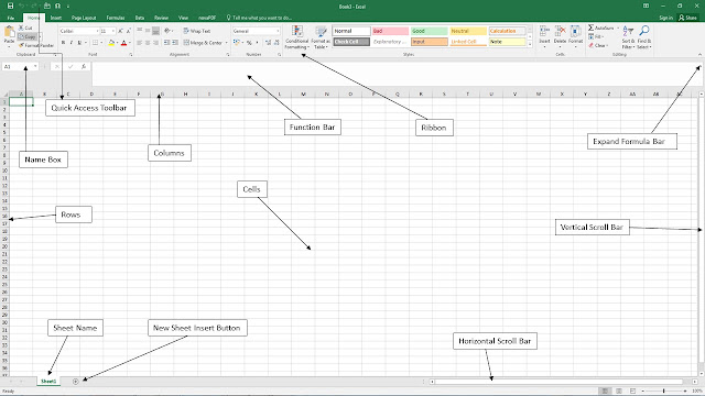
Exploring the Microsoft Excel Interface

EXPLORING THE MICROSOFT EXCEL INTERFACE


When you start Microsoft Excel you can see similar interface as per shown in below image.


Exploring The Microsoft Excel Interface

Microsoft Excel Shortcut Keys


Microsoft Excel Shortcut Keys


DESCRIPTION OF SHORTCUT SHORTCUT KEYS
Open New Excel Workbook CTRL + N
Create New Sheet ALT + SHIFT + F1
Open File CTRL + F12
Save workbook CTRL + S
Save As F12
Copy CTR L+ C
Pest CTRL + V
Bold CTRL + B OR CTRL + @
Italic CTRL + I OR CTRL + #
Underline CTRL + U OR CTRL + $
Strikethrough Example CTRL + %
Quik Open Font Format Cell CTRL + SHIFT + F
Copy Above Cell CTRL + D
Print CTRL + P
Undo CTRL + Z
Redo CTRL + Y
All Borders First Select cells Range and press ALT + H + B + A
Outside Borders First Select cells Range and press ALT + H + B + S
Remove All Borders First Select cells Range and press ALT + H + B + N
Merge and Center Cells First Select cells Range and press ALT + H + M + C
Merge Cells First Select cells Range and press ALT + H + M + M
Unmerge Cells First Select cells Range and press ALT + H + M + U
Value Pest First copy text that you want & press ALT + E + S + V
Format Pest First copy format that you want & press ALT + E + S + T
Coment Pest First copy commet that you want & press ALT + E + S + C
Formula Pest First copy formula that you want & press ALT + E + S + F
Find CTRL + F
Replace CTRL + F > ALT + P
Close Existing Excel Workbook ALT + F + C or ALT F4
Close All Excel Workbook ALT + F + X
Move between multipal Workbook ALT + Tab
Move between multipal sheet
CTRL + Page Down to move forward
CTRL + Page Up to move Backward
Write below in same cell  First select cell and press ALT + ENTER
Go to End CTRL + End
Go to A1 Cell CTRL + Home
Go to Up in Existing Columns CTRL + Up key
Go to Down in Existing Columns CTRL + Down key
Go to Left in Existing Rows CTRL + Left key
Go to Right in Existing Rows CTRL + Right key
Select All CTRL + A
Select Column CTRL + Space bar
Select Rows Shift + Space bar
Add Column CTRL + Space bar and CTRL + (+) Button
Add Rows Shift + Space bar and CTRL + (+) Button
Delete Column CTRL + Space bar and CTRL + (-) Button
Delete Rows Shift + Space bar and CTRL + (-) Button
Hide Column CTRL + )
Hide Row CTRL + (
Go to Any cell CTRL + G and type cell no in reference and press enter or F5
Take Screen Shot CTRL + Print Screen and pest where you want
Apply Filter Shift + Space Bar and press CTRL + SHIFT + L
Remove Filter Shift + Space Bar and press CTRL + SHIFT + L
Sum First go at the end of the number list and press Alt + (=) button and press enter
Auto Adjust Column Width CTRL + Space Bar and ALT + O + C + A
Auto Adjust Row Width Shift + Space Bar and ALT + O + R + A
Show All formula in Sheet CTRL + ` OR CTRL + ~
Quik Open Number Format Cell CTRL + !
Open help Menu F1
Edit Selected Cell F2
Pest Cell Name F3
Repeat Last Action F4 Ex. If you change colour of any cell and you want to repeat same action in other cell press F4
Spelling Check F7
Move to Next Pane F6
Enter Extend Mode F8
Recalculate Every Workbook F9
Activate Menu Bar F10
Create Chart form Selected Data F11
Insert Chart ALT + F1
Minimize Current Window CTRL + F9
Restore Down or Maximize Current Window CTRL + F10
Previous Workbook CTRL + SHIFT +F6
Next Workbook CTRL + F6